AMBER
Adapted from AMBER tutorial. Read the full manual. See github for exmple scripts.
Introduction
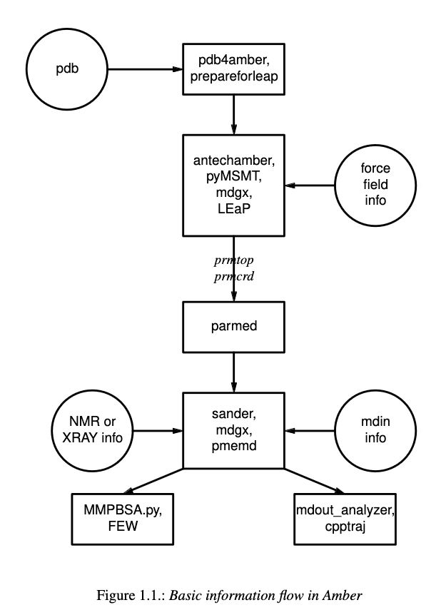
AMBER is a suite of molecular dynamics programs that can be used to simulate
biomolecules at a variety of granularities. It is broken into two main parts.
AMBERTools, which includes the free-to-use MD engine, sander which runs on
CPUs, as well as various analysis scripts. And AMBER, which is distributed
through a license and includes the GPU-accelerated engine, pmemd. We will
be using the pmemd version of the software.
All-atom with explicit solvent
The most common (and likely accurate) type of simulation is all-atom with explicit solvent. In this simulation, all atoms, including solvent molecules are simulated as discrete points.
Prepare structure
The first step to any simulation is to acquire a starting structure. We will usually start from a PDB, either a solved structure, one you’ve modelled, or one that you’ve built. Things to consider with making a starting structure:
the larger the system the longer the simulation steps will take
clashes need to be resolved or they will cause failures later
most of the time, it’s best to remove 5’ phosphates from DNA
For this tutorial, we will start from a github repo (clone this in your PL)
biokem-interactive
cd <test_location>
git clone https://github.com/Luger-Lab/MD-simulations.git
This repo is organized first by type of simulation, type of solvent, where
this simulation will run, and finally by replicate number. When running this for real,
clone a new repo and then copy the rep0 directory into one with the unique
identifier of your simulation. But for now, navigate to the
all_atom/explicit_solvent/blanca/rep0:
cd MD-simulations/all_atom/explicit_solvent/blanca/rep0
If you ls this directory, you should see all of the necessary directories for
running a simulation:
analysis: contains scripts and is a place to run/store analysis
mdinfo: empty, but will contain simple information about your run
outputs: empty, but will contain detailed information about your run
pdb_prep: contains example pdb, get your structure ready here
restarts: empty, but will contain snapshots used to “restart” simulations
scripts: contains most of the scripts you will need to run
trajectories: empty, but will contain the actual data files
Navigate to the pdb_prep directory and open the example pdb:
cd pdb_prep
sbgrid
chimerax atg.pdb
You should see a simple three basepair DNA strand. With your own starting structure, now is the time to resolve clashes, remove any 5’ phosphates, and make sure residues are named properly (DNA needs to be DA, DC, DT, DG). But we will exit ChimeraX and prep the pdb. We will load the AMBER module and use a contained program to reduce the system, remove waters, and put the file in the correct format. Although this step isn’t always necessary, it’s usually helpful.
ml amber
pdb4amber -i atg.pdb -o atg_amber.pdb --reduce --dry
If there were no errors, the output should say so and should have created a number of files. We can now add enough ions to the system to neutralize it (a non-neutral system creates potentials which are often to large to calculate). We will need to edit this file:
#load forcefield parameters
source leaprc.protein.ff14SB
source leaprc.DNA.bsc1
source leaprc.water.tip3p

unit = loadpdb <name>.pdb
#'loadpbd' fills in missing H atoms, and missing heavy atoms

#add counter-ions
addions unit Cl- 0
addions unit K+ 0

#save neutralized PDB
savepdb unit <name>_neutralized.pdb

quit
In this file, we will load the various forcefields we need (there are other forcefields for different molecules, as well as different versions of each). We will then load our pdb, add counterions and save the pdb. Edit this file with the correct input and output filenames:
nano ../scripts/0_neutralize.leap
You can now run the file using a program called tleap (from pdb_prep):
tleap -sf ../scripts/0_neutralize.leap
If all goes well, you should get 0 errors and a readout telling which ions were placed.
We will now edit the next scripts and look at how many water molecules we need to solvate our box:
nano ../scripts/1_addwater.leaptleap -sf ../scripts/1_addwater.leap
We can take the number of residues add (waters) and run:
python ../scripts/2_salt_concentration.py --wat <waters> --conc <molarity_of_salt>
You can place the output of this into the next script (don’t forget to edit the names and box size as well):
nano ../scripts/3_addions.leap
Run with tleap:
tleap -sf ../scripts/3_addions.leap
To speed up the simulation we will reparition the mass of hydrogen atoms, which allows us to run longer time steps.
parmed -p nhmrp_atg_buffer.prmtopHMassRepartitionoutparm ../atg_buffer.prmtop quit
Minimization
Now we have prepared our system and can run a minimization step to relieve any
atom placements that may cause problems later. We will run the rest of our scripts
from the scripts directory:
cd ../scripts
We will use two input files to run minimization:
min1.in:
Minimization 1
&cntrl
imin=1,maxcyc=5000,irest=0,ntx=1,
ntpr=5,
ntr=1, restraint_wt=10.0,restraintmask='(!:WAT,Cl-,Na+,NA,CL,K+,K)&!(@H=)',
cut=10.0,ntt=3,gamma_ln=3,temp0=10.0,
ntb=1,iwrap=1,
/

&ewald
vdwmeth=1,order=4,dsum_tol=0.000001,netfrc=0,eedmeth=1,
/
min2.in:
Minimization 2
&cntrl
imin=1,maxcyc=5000,irest=0,ntx=1,
ntpr=5,
cut=10.0,ntt=3,gamma_ln=3,temp0=10.0,
ntb=1,iwrap=1,
/

&ewald
vdwmeth=1,order=4,dsum_tol=0.000001,netfrc=0,eedmeth=1,
/
In the first minimization we are restraining anything that isn’t part of the buff to allow the buffer to disperse in the box. In the second, we are allowing the whole system to disperse. We will run this script on the cluster with (you will need to edit and fill in the name of your system):
4_blanca_minimization.q:
#!/bin/bash
#SBATCH --partition=blanca-biokem
#SBATCH --qos=blanca-biokem
#SBATCH --account=blanca-biokem
#SBATCH --job-name=minimization
#SBATCH --nodes=1
#SBATCH --ntasks=50
#SBATCH --mem=128gb
#SBATCH --time=24:00:00
#SBATCH --output=/home/%u/slurmfiles_out/slurm_%j.out
#SBATCH --error=/home/%u/slurmfiles_err/slurm_%j.err

module load amber/v22
NAME=''

#run the first minimization
mpirun -np 50 pmemd.MPI -O -i min1.in -o ../outputs/min1.out -p ../${NAME}_buffer.prmtop -c ../${NAME}_buffer.inpcrd -r ../restarts/${NAME}_min1.rst\
-x ../trajectories/${NAME}_min1.nc -inf ../mdinfo/${NAME}_min1.mdinfo -ref ../${NAME}_buffer.inpcrd

#run the second minimization
mpirun -np 50 pmemd.MPI -O -i min2.in -o ../outputs/min2.out -p ../${NAME}_buffer.prmtop -c ../restarts/${NAME}_min1.rst -r ../restarts/${NAME}_min2.rst\
-x ../trajectories/${NAME}_min2.nc -inf ../mdinfo/${NAME}_min2.mdinfo
Run these minimizations on the cluster:
sbatch 4_blanca_minimization.q
You can check the progress of the run by reading the files in mdinfo and
outputs. This step could take ~1 hour, depending on the size of the system.
If there are unresolved clashes in your system, it make take longer or run out
of memory and fail, in which case you will need to go back to the starting structure,
resolve clashes and start over.
Heating
Up until this point, no random numbers have been applied to the simulation, meaning that if you were to repeat this process with the same starting structure, you should get the exact same setup out. But in the heating step, we actually start to use random numbers to assign starting velocities. In this way, we can treat separate runs as replicates, which allows us (in theory) to sample more conformational space. The other commonly used method to do this is to run the simulation for a very long time, there is much debate about which method is better.
There’s no need to rerun the previous steps when making replicates, we can simply copy the whole directory.
cp -r ../../rep0 ../../rep1
cp -r ../../rep0 ../../rep2
Because the starting molecule is usually a crystal structure or other idealized low energy state, it has a temperature of almost 0K. But we want to run the system at a more realistic temperature (usually ~300K, but it can be a value of your choosing). To add kinetic energy to the systerm without having it fly apart, we will heat it up slowly and restrain the motion of the macromolecules. The input file looks like this:
heat.in:
Heat
  &cntrl
   ig=-1,imin=0,irest=0,ntx=1,nstlim=12500,dt=0.004,
   ntwx=2500,ioutfm=1,ntpr=2500,ntwr=2500,
   ntt=3,gamma_ln=3.0,tempi=10.0,temp0=300.0,
   ntc=2,ntf=2,cut=10.0,
   ntr=1,restraint_wt=10.0,restraintmask="(!:WAT,Na+,Cl-,K+,K,NA,CL)&!(@H=)",
   ntb=1,iwrap=1,
   nmropt=0,
  /

  &wt type='END',
  /
We will run it and the equilibration step at the same time.
Equilibration
After heating up the solvent and restrained macromolecules, we will slowly release the restrains on the macromolecules to bring the system up to 300K and 1atm.
release1.in:
Release 1
  &cntrl
   ig=-1,imin=0,irest=1,ntx=5,nstlim=25000,dt=0.004,
   ntwx=2500,ioutfm=1,ntpr=2500,ntwr=2500,
   ntt=3,gamma_ln=3.0,temp0=300.0,
   ntb=2,iwrap=1,ntp=1,barostat=2,pres0=1.01325,taup=3.0,
   ntc=2,ntf=2,cut=10.0
   ntr=1,restraint_wt=10.0,restraintmask="(!:WAT,Na+,Cl-,NA,CL,K+,K)&(!(@H=))",
   nmropt=0,
  /

  &ewald
   vdwmeth=1,order=4,dsum_tol=0.000001,eedmeth=1,
  /
release2.in:
Release 2
  &cntrl
   ig=-1,imin=0,irest=1,ntx=5,nstlim=25000,dt=0.004,
   ntwx=2500,ioutfm=1,ntpr=2500,ntwr=2500,
   ntt=3,gamma_ln=3.0,temp0=300.0,
   ntb=2,iwrap=1,ntp=1,barostat=2,pres0=1.01325,taup=3.0,
   ntc=2,ntf=2,cut=10.0
   ntr=1,restraint_wt=3.0,restraintmask="(!:WAT,Na+,Cl-,NA,CL,K+,K)&(!(@H=))",
   nmropt=0,
  /

  &ewald
   vdwmeth=1,order=4,dsum_tol=0.000001,eedmeth=1,
  /
release3.in
Release 3
  &cntrl
   ig=-1,imin=0,irest=1,ntx=5,nstlim=25000,dt=0.004,
   ntwx=2500,ioutfm=1,ntpr=2500,ntwr=2500,
   ntt=3,gamma_ln=3.0,temp0=300.0,
   ntb=2,iwrap=1,ntp=1,barostat=2,pres0=1.01325,taup=3.0,
   ntc=2,ntf=2,cut=10.0
   ntr=1,restraint_wt=1.0,restraintmask="(!:WAT,Na+,Cl-,NA,CL,K+,K)&(!(@H=))",
   nmropt=0,
  /

  &ewald
   vdwmeth=1,order=4,dsum_tol=0.000001,eedmeth=1,
  /
release4.in:
Release 4
  &cntrl
   ig=-1,imin=0,irest=1,ntx=5,nstlim=25000,dt=0.004,
   ntwx=2500,ioutfm=1,ntpr=2500,ntwr=2500,
   ntt=3,gamma_ln=3.0,temp0=300.0,
   ntb=2,iwrap=1,ntp=1,barostat=2,pres0=1.01325,taup=3.0,
   ntc=2,ntf=2,cut=10.0
   ntr=1,restraint_wt=0.3,restraintmask="(!:WAT,Cl-,Na+,CL,NA,K+,K)&(!(@H=))",
   nmropt=0,
  /

  &ewald
   vdwmeth=1,order=4,dsum_tol=0.000001,eedmeth=1,
  /

  DISANG=./inputs/fraying.RST
  DUMPAVE=./outputs/thisrun_fraying.dat
  LISTIN=POUT
  LISTOUT=POUT
release5.in:
Release 5
  &cntrl
   ig=-1,imin=0,irest=1,ntx=5,nstlim=25000,dt=0.004,
   ntwx=2500,ioutfm=1,ntpr=2500,ntwr=2500,
   ntt=3,gamma_ln=3.0,temp0=300.0,
   ntb=2,iwrap=1,ntp=1,barostat=2,pres0=1.01325,taup=3.0,
   ntc=2,ntf=2,cut=10.0
   ntr=1,restraint_wt=0.1,restraintmask="(!:WAT,Na+,Cl-,NA,CL,K+,K)&(!(@H=))",
   nmropt=0,
  /

  &ewald
   vdwmeth=1,order=4,dsum_tol=0.000001,eedmeth=1,
  /
We can run this and the heating step by editing and running
5_blanca_heat_and_density_equilibrate.q:
#!/bin/bash
#SBATCH --partition=blanca-biokem
#SBATCH --qos=blanca-biokem
#SBATCH --account=blanca-biokem
#SBATCH --job-name=md_heat_and_eq
#SBATCH --nodes=1
#SBATCH --gres=gpu:1
#SBATCH --ntasks=1
#SBATCH --mem=128gb
#SBATCH --time=24:00:00
#SBATCH --output=/home/%u/slurmfiles_out/slurm_%j.out
#SBATCH --error=/home/%u/slurmfiles_err/slurm_%j.err

module load amber/v22
NAME=''

pmemd.cuda -O -i heat.in \
            -o ../outputs/${NAME}_heat.out \
            -p ../${NAME}_buffer.prmtop \
            -c ../restarts/${NAME}_min2.rst \
            -r ../restarts/${NAME}_heat.rst \
            -x ../trajectories/${NAME}_heat.nc \
            -inf ../mdinfo/${NAME}_heat.mdinfo \
            -ref ../restarts/${NAME}_min2.rst

pmemd.cuda -O -i release1.in \
            -o ../outputs/${NAME}_release1.out \
            -p ../${NAME}_buffer.prmtop \
            -c ../restarts/${NAME}_heat.rst \
            -r ../restarts/${NAME}_release1.rst \
            -x ../trajectories/${NAME}_release1.nc \
            -inf ../mdinfo/${NAME}_release1.mdinfo \
            -ref ../restarts/${NAME}_heat.rst

pmemd.cuda -O -i release2.in \
            -o ../outputs/${NAME}_release2.out \
            -p ../${NAME}_buffer.prmtop \
            -c ../restarts/${NAME}_release1.rst \
            -r ../restarts/${NAME}_release2.rst \
            -x ../trajectories/${NAME}_release2.nc \
            -inf ../mdinfo/${NAME}_release2.mdinfo \
            -ref ../restarts/${NAME}_release1.rst

pmemd.cuda -O -i release3.in \
            -o ../outputs/${NAME}_release3.out \
            -p ../${NAME}_buffer.prmtop \
            -c ../restarts/${NAME}_release2.rst \
            -r ../restarts/${NAME}_release3.rst \
            -x ../trajectories/${NAME}_release3.nc \
            -inf ../mdinfo/${NAME}_release3.mdinfo \
            -ref ../restarts/${NAME}_release2.rst

pmemd.cuda -O -i release4.in \
            -o ../outputs/${NAME}_release4.out \
            -p ../${NAME}_buffer.prmtop \
            -c ../restarts/${NAME}_release3.rst \
            -r ../restarts/${NAME}_release4.rst \
            -x ../trajectories/${NAME}_release4.nc \
            -inf ../mdinfo/${NAME}_release4.mdinfo \
            -ref ../restarts/${NAME}_release3.rst

pmemd.cuda -O -i release5.in \
            -o ../outputs/${NAME}_release5.out \
            -p ../${NAME}_buffer.prmtop \
            -c ../restarts/${NAME}_release4.rst \
            -r ../restarts/${NAME}_release5.rst \
            -x ../trajectories/${NAME}_release5.nc \
            -inf ../mdinfo/${NAME}_release5.mdinfo \
            -ref ../restarts/${NAME}_release4.rst
Run using:
sbatch 5_blanca_heat_and_density_equilibrate.q
Production
If the last step ran properly, we now have a system read to be simulated. We can
use the time estimation in mdinfo to estimate how many time steps we can run
before hitting the wallclock limit on the cluster (usually 24hrs). We will simulate
the first 50ns, from there you can simply copy that entry, edit, and run longer.
We will run 25ns runs, using a 4fs time step as specified in 25ns_4fs_per_step.in:
Benchmark
  &cntrl
   ig=-1,imin=0,irest=1,ntx=5,nstlim=6250000,dt=0.004,
   ntwx=2500,ioutfm=1,ntpr=2500,ntwr=2500,
   ntt=3,gamma_ln=3.0,temp0=300.0,
   ntb=2,iwrap=1,ntp=1,barostat=2,pres0=1.01325,taup=3.0,
   ntc=2,ntf=2,cut=10.0
  /

  &ewald
   vdwmeth=1,order=4,dsum_tol=0.000001,eedmeth=1,
  /
Using 6_blanca_production_50ns.q:
#!/bin/bash
#SBATCH --partition=blanca
#SBATCH --qos=preemptable
#SBATCH --account=blanca-biokem
#SBATCH --job-name=md_sim_50ns
#SBATCH --nodes=1
#SBATCH --gres=gpu:1
#SBATCH --ntasks=1
#SBATCH --mem=128gb
#SBATCH --time=24:00:00
#SBATCH --output=/home/%u/slurmfiles_out/slurm_%j.out
#SBATCH --error=/home/%u/slurmfiles_err/slurm_%j.err

module load amber/v22
NAME=''

pmemd.cuda -O -i 25ns_4fs_per_step.in \
            -o ../outputs/${NAME}_25ns.out \
            -p ../${NAME}_buffer.prmtop \
            -c ../restarts/${NAME}_release5.rst \
            -r ../restarts/${NAME}_25ns.rst \
            -x ../trajectories/${NAME}_25ns.nc \
            -inf ../mdinfo/${NAME}_25ns.mdinfo


pmemd.cuda -O -i 25ns_4fs_per_step.in \
            -o ../outputs/${NAME}_50ns.out \
            -p ../${NAME}_buffer.prmtop \
            -c ../restarts/${NAME}_25ns.rst \
            -r ../restarts/${NAME}_50ns.rst \
            -x ../trajectories/${NAME}_50ns.nc \
            -inf ../mdinfo/${NAME}_50ns.mdinfo
Submit using:
sbatch 6_blanca_production_50ns.q
Analysis
Vizualizing trajectories
Chimera
We can view the system in Chimera by opening the application (best done on viz node):
sbgrid
chimera
Then load you prmtop and nc files:
Tools > MD/Ensemble Analysis > MD Movie
You target of interest will move around as time goes on. To center it, select the
molecule and click Actions > Hold Steady in the MD movie dialog box. You may
also want to change the step size of your playback.
While there are many types of analyses that can be done on MD simulations, tracking RMSD over time and calculating the ∆G of a ligand-receptor.
ChimeraX
sbgrid
chimerax
In ChimeraX:
open <name>_neutralized.pdb
open <path to trajectory> structureModel #1
set bgColor white; hide protein atoms; show nucleic cartoon; nucleotides ladder; color nucleic #aaaaaa; color protein #ffb347; lighting soft; graphics silhouettes width 1.5; nucleotides tube/slab shape box; view
coordset slider #1
Record movie example:
movie record; coordset #1 1,30000,100 holdSteady @ca; wait 310; movie encode D:/shawn/md_movies/0M_hpya_tetra_nuc_300ns.mp4
RMSD over time
∆G of ligand-receptor
All-atom with implicit solvent
Preparing structures with implicit solvents requires that we use the igb=8 parameter
as well as remove the periodic box argument. Because we aren’t using solvent,
we also don’t need to solvate the system.
The rest of the simulation continues like the explicit solvent.
Coarse-grained (implicit solvent)
Prepare structure
The major difference in performing a coarse-grained simulation is converting residues into beads of average charge and mass, which approximate the properties of the residues they are standing in for. We will use the SIRAH forcefields and conversion tools to do this.
Production
The major difference in the production step is that instead of simulating on the order of 10s of ns, you can simulate on the microsecond timescale.